Hamiltonian Dynamics of the Ising Model

In this example, we simulate Hamiltonian Dynamics of the Transverse Field Ising Model (TFIM). The model is defined by the Hamiltonian

$$ H = -J\sum_{(i,j)\in E}Z_iZ_j + B\sum_{i\in V}X_i $$

for a lattice graph \(G=(V,E)\) and real parameters \(J, B\). We investigate the total magnetization

$$ M = \sum_{i\in V}Z_i $$

of the system of qubits as it evolves under the Hamiltonian.

Here, we consider an Ising chain:

import matplotlib.pyplot as plt
import networkx as nx
import numpy as np

def generate_chain_graph(N):
    coupling_list = [[k,k+1] for k in range(N-1)]
    G = nx.Graph()
    G.add_edges_from(coupling_list)
    return G

G = generate_chain_graph(6)

First, we implement methods for creating the Ising Hamiltonian and the total magnetization observable for a given graph.

from qrisp import QuantumVariable
from qrisp.operators import X, Y, Z

def create_ising_hamiltonian(G, J, B):
    H = sum(-J*Z(i)*Z(j) for (i,j) in G.edges()) + sum(B*X(i) for i in G.nodes())
    return H

def create_magnetization(G):
    H = (1/G.number_of_nodes())*sum(Z(i) for i in G.nodes())
    return H

With all the necessary ingredients, we conduct the experiment: For varying evolution times \(T\):

• Prepare the state \(\psi(t)=e^{-itH}\ket{0}^{\otimes N}\) by performing Hamiltonian simulation via Trotterization.

• Measure the total magnetization \(\langle\psi(t)|M|\psi(t)\rangle\).

T_values = np.arange(0, 2.0, 0.05)
M_values = []

H = create_ising_hamiltonian(G,1.0,1.0)
U = H.trotterization()
M = create_magnetization(G)

def psi(t):
    qv = QuantumVariable(G.number_of_nodes())
    U(qv,t=t,steps=5)
    return qv

for t in T_values:

    magnetization = M.expectation_value(psi, precision=0.005)(t)
    M_values.append(magnetization)

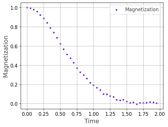
Finally, we visualize the results. As expected, the total magnetization decreases in the presence of a transverse field with increasing evolution time \(T\).

import matplotlib.pyplot as plt
plt.scatter(T_values, M_values, color='#6929C4', marker="o", linestyle="solid", s=20, label=r"Ising chain")
plt.xlabel(r"Evolution time $T$", fontsize=15, color="#444444")
plt.ylabel(r"Magnetization $\langle M \rangle$", fontsize=15, color="#444444")
plt.legend(fontsize=15, labelcolor="#444444")
plt.tick_params(axis='both', labelsize=12)
plt.grid()
plt.show()