VQEProblem#

class VQEProblem(hamiltonian, ansatz_function, num_params, init_function=None, callback=False)[source]#

Central structure to facilitate treatment of VQE problems. This class encapsulates the Hamiltonian, the ansatz, and the initial state preparation function for a specific VQE problem instance.

Parameters:

hamiltonianQubitOperator or FermionicOperator: The problem Hamiltonian.
ansatz_functioncallable: A function receiving a QuantumVariable, and an array of real parameters of size (n,). This function implements the unitary corresponding to one layer of the ansatz.
num_paramsint: The number of parameters \(n\) per layer of the ansatz.
init_functioncallable, optional: A function receiving a QuantumVariable and preparing the initial state from the \(\ket{0}\) state. By default, the inital state is the \(\ket{0}\) state.
callbackbool, optional: If True, intermediate results are stored. The default is False.

Examples

For a quick demonstration, we show how to calculate the ground state energy of the \(H_2\) molecule using VQE. The electronic_structure_problem method generates a VQEProblem instance with the Hamiltonian and a chemistry-inspired Qubit Coupled Cluster Single Double (QCCSD) ansatz.

from pyscf import gto
from qrisp import QuantumVariable
from qrisp.vqe.problems.electronic_structure import *

mol = gto.M(
    atom = '''H 0 0 0; H 0 0 0.74''',
    basis = 'sto-3g')

vqe = electronic_structure_problem(mol)

energy = vqe.run(QuantumVariable(4), depth=1, max_iter=50)
print(energy)
#Yields -1.8461290172512965

You can also specify a custom Hamiltonian and a custom hardware-efficient ansatz, as explained here.

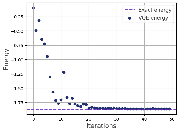
from qrisp import *
from qrisp.operators.qubit import X,Y,Z

# Problem Hamiltonian
c = [-0.81054, 0.16614, 0.16892, 0.17218, -0.22573, 0.12091, 0.166145, 0.04523]
H = c[0] \
    + c[1]*Z(0)*Z(2) \
    + c[2]*Z(1)*Z(3) \
    + c[3]*(Z(3) + Z(1)) \
    + c[4]*(Z(2) + Z(0)) \
    + c[5]*(Z(2)*Z(3) + Z(0)*Z(1)) \
    + c[6]*(Z(0)*Z(3) + Z(1)*Z(2)) \
    + c[7]*(Y(0)*Y(1)*Y(2)*Y(3) + X(0)*X(1)*Y(2)*Y(3) + Y(0)*Y(1)*X(2)*X(3) + X(0)*X(1)*X(2)*X(3))

# Ansatz
def ansatz(qv,theta):
    for i in range(4):
        ry(theta[i],qv[i])
    for i in range(3):
        cx(qv[i],qv[i+1])
    cx(qv[3],qv[0])

from qrisp.vqe.vqe_problem import *

vqe = VQEProblem(hamiltonian = H,
                 ansatz_function = ansatz,
                 num_params = 4,
                 callback = True)

energy = vqe.run(QuantumVariable(4),
              depth = 1,
              max_iter = 50)
print(energy)
# Yields -1.864179046

Note that for comparing to the results in the aforementioned paper, we have to add the nuclear repulsion energy \(E_{\text{nuc}}=0.72\) to the calculated electronic energy \(E_{\text{el}}\).

We visualize the optimization process:

>>> vqe.visualize_energy(exact=True)

Methods#

`VQEProblem.set_init_function`(init_function)	Set the initial state preparation function for the VQE problem.
`VQEProblem.run`(qarg, depth[, mes_kwargs, ...])	Run VQE for the specific problem instance.
`VQEProblem.train_function`(qarg, depth[, ...])	This function allows for training of a circuit with a given instance of a `VQEProblem`.
`VQEProblem.compile_circuit`(qarg, depth)	Compiles the circuit that is evaluated by the `run` method.
`VQEProblem.benchmark`(qarg, depth_range, ...)	This method enables convenient data collection regarding performance of the implementation.
`VQEProblem.visualize_energy`([exact])	Visualizes the energy during the optimization process.