Quantum Imaginary-Time Evolution

QITE(qarg, U_0, exp_H, s, k)

Performs Double-Braket Quantum Imaginary-Time Evolution (DB-QITE) via implementing the unitary \(U_k\) that is defined recursively by

\[U_{k+1} = e^{i\sqrt{s_k}H}U_ke^{i\sqrt{s_k}\ket{0}\bra{0}}U_k^{\dagger}e^{-i\sqrt{s_k}H}U_k\]

where \(H\) is the Hamiltonian Operator.

Parameters:

qargQuantumVariable or QuantumArray

The quantum argument on which quantum imaginary time evolution is performed.

U_0function

A Python function that takes a QuantumVariable or QuantumArray qarg as input, and prepares the initial state.

exp_Hfunction

A Python function that takes a QuantumVariable or QuantumArray qarg and time t as input, and performs forward evolution \(e^{-itH}\).

slist[float] or list[Sympy.Symbol]

A list of evolution times for each step.

kint

The number of steps.

Examples

We utilize QITE to approximate the ground state energy of a Heisenberg chain. We start by defining the lattice graph \(G\):

import networkx as nx

# Create a graph
N = 4
G = nx.Graph()
G.add_edges_from([(k,k+1) for k in range(N-1)]) 

Next, we set up the Heisenberg Hamiltonian and calculate the ground state energy classically:

from qrisp.operators import X, Y, Z

def create_heisenberg_hamiltonian(G):
    H = sum(X(i)*X(j)+Y(i)*Y(j)+Z(i)*Z(j) for (i,j) in G.edges())
    return H

H = create_heisenberg_hamiltonian(G)
print(H)
print(H.ground_state_energy())

As explained in this example, a suitable initial approximation for the ground state is given by a tensor product of singlet states \(\frac{1}{\sqrt{2}}(\ket{10}-\ket{01})\) corresponding to a maximal matching of the graph \(G\). Accordingly, we define the function U_0:

from qrisp import QuantumVariable   
from qrisp.vqe.problems.heisenberg import create_heisenberg_init_function

M = nx.maximal_matching(G)
U_0 = create_heisenberg_init_function(M)

qv = QuantumVariable(N)
U_0(qv)
E_0 = H.get_measurement(qv)
print(E_0)

For the function exp_H that performs forward evolution \(e^{-itH}\), we use the trotterization method with 5 Trotter steps:

def exp_H(qv, t):
    H.trotterization(method='commuting')(qv,t,5)

With all the necessary ingredients, we use QITE to approximate the ground state:

import numpy as np
import sympy as sp
from qrisp.qite import QITE

steps = 4
s_values = np.linspace(.01,.3,10)

theta = sp.Symbol('theta')
optimal_s = [theta]
optimal_energies = [E_0]

for k in range(1,steps+1):

    # Perform k steps of QITE
    qv = QuantumVariable(N)
    QITE(qv, U_0, exp_H, optimal_s, k)
    qc = qv.qs.compile()

    # Find optimal evolution time 
    # Use "precompliled_qc" keyword argument to avoid repeated compilation of the QITE circuit
    energies = [H.get_measurement(qv,subs_dic={theta:s_},precompiled_qc=qc,diagonalisation_method='commuting') for s_ in s_values]
    index = np.argmin(energies)
    s_min = s_values[index]

    optimal_s.insert(-1,s_min)
    optimal_energies.append(energies[index])

print(optimal_energies)

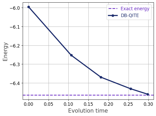
Finally, we visualize the results:

import matplotlib.pyplot as plt

evolution_times = [sum(optimal_s[i] for i in range(k)) for k in range(steps+1)]

plt.xlabel('Evolution time', fontsize=15, color='#444444')
plt.ylabel('Energy', fontsize=15, color='#444444')
plt.axhline(y=H.ground_state_energy(), color='#6929C4', linestyle='--', linewidth=2, label='Exact energy')
plt.plot(evolution_times, optimal_energies, c='#20306f', marker="o", linestyle='solid', linewidth=3, zorder=3, label='DB-QITE')
plt.legend(fontsize=12, labelcolor='linecolor')
plt.tick_params(axis='both', labelsize=12)
plt.grid()
plt.show()

In the Examples, we also show how to solve MaxCut with QITE.