qrisp.gqsp.hamiltonian_simulation#

hamiltonian_simulation(H: BlockEncoding | FermionicOperator | QubitOperator, t: ArrayLike = 1, N: int = 1) → BlockEncoding[source]#

Returns a BlockEncoding approximating Hamiltonian simulation of the operator.

For a block-encoded Hamiltonian \(H\), this method returns a BlockEncoding of an approximation of the unitary evolution operator \(e^{-itH}\) for a given time \(t\).

The approximation is based on the Jacobi-Anger expansion into Bessel functions of the first kind (\(J_n\)):

\[e^{-it\cos(\theta)} \approx \sum_{n=-N}^{N}(-i)^nJ_n(t)e^{in\theta}\]

Parameters:

HBlockEncoding | FermionicOperator | QubitOperator: The Hermitian operator to be simulated.
tArrayLike: The scalar evolution time \(t\). The default is 1.0.
Nint: The truncation order \(N\) of the expansion. A higher order provides better approximation for larger \(t\) or higher precision requirements. Default is 1.

Returns:

BlockEncoding: A new BlockEncoding instance representing an approximation of the unitary \(e^{-itH}\).

Notes

Precision: The truncation error scales (decreases) super-exponentially with \(N\). For a fixed \(t\), choosing \(N > |t|\) ensures rapid convergence.
Normalization: The resulting operator is nearly unitary, meaning its block-encoding normalization factor \(\alpha\) will be close to 1.

References

Low & Chuang (2019) Hamiltonian Simulation by Qubitization.
Motlagh & Wiebe (2024) Generalized Quantum Signal Processing.

Examples

Below is an example of using the hamiltonian_simulation() function to simulate a quantum system governed by an Ising Hamiltonian on a 1D chain graph. In this example, we construct a chain graph, define an Ising Hamiltonian with specific coupling and magnetic field strengths, and compute the system’s energy and magnetization over various evolution times using the QSP-based simulation algorithm. Finally, the results are compared against a classical simulation.

import matplotlib.pyplot as plt
import networkx as nx
import numpy as np
from qrisp import *
from qrisp.gqsp import hamiltonian_simulation
from qrisp.operators import X, Y, Z
import scipy as sp

def generate_chain_graph(N):
    coupling_list = [[k,k+1] for k in range(N-1)]
    G = nx.Graph()
    G.add_edges_from(coupling_list)
    return G

def create_ising_hamiltonian(G, J, B):
    H = sum(-J * Z(i) * Z(j) for (i,j) in G.edges()) + sum(B * X(i) for i in G.nodes())
    return H

def create_magnetization(G):
    H = (1 / G.number_of_nodes()) * sum(Z(i) for i in G.nodes())
    return H

# Evaluate observables classically
def sim_classical(T_values, H, M):
    M_values = []
    E_values = []
    H_mat = H.to_array()
    M_mat = M.to_array()

    def _psi(t):
        psi0 = np.zeros(2**H.find_minimal_qubit_amount())
        psi0[0] = 1
        psi = sp.linalg.expm(-1.0j * t * H_mat) @ psi0
        psi = psi / np.linalg.norm(psi)
        return psi

    for t in T_values:
        psi = _psi(t)
        magnetization = (np.conj(psi) @ M_mat @ psi).real
        energy = (np.conj(psi) @ H_mat @ psi).real
        M_values.append(magnetization)
        E_values.append(energy)

    return np.array(M_values), np.array(E_values)

# Evaluate observables using QSP-based simulation
def sim_qsp(T_values, H, M):
    M_values = []
    E_values = []

    def operand_prep():
        return QuantumFloat(H.find_minimal_qubit_amount())

    def psi(t):
        BE = hamiltonian_simulation(H, t=t, N=10)
        operand = BE.apply_rus(operand_prep)()
        return operand

    @jaspify(terminal_sampling=True)
    def magnetization(t):
        magnetization = M.expectation_value(psi, precision=0.005)(t)
        return magnetization

    @jaspify(terminal_sampling=True)
    def energy(t):
        energy = H.expectation_value(psi, precision=0.005)(t)
        return energy

    for t in T_values:
        M_values.append(magnetization(t))
        E_values.append(energy(t))

    return np.array(M_values), np.array(E_values)

G = generate_chain_graph(6)
H = create_ising_hamiltonian(G, 0.25, 0.5)
M = create_magnetization(G)

T_values = np.arange(0.1, 3.0, 0.1)
M_classical, E_classical = sim_classical(T_values, H, M)
M_qsp, E_qsp = sim_qsp(T_values, H, M)

# Plot the results
plt.scatter(T_values, E_classical, color='#20306f', marker="d", label="E target")
plt.scatter(T_values, M_classical, color='#6929C4', marker="d", label="M target")
plt.plot(T_values, E_qsp, color='#20306f', marker="o", linestyle="solid", alpha=0.5, label="E qsp")
plt.plot(T_values, M_qsp, color='#6929C4', marker="o", linestyle="solid", alpha=0.5, label="M qsp")
plt.xlabel("Evolution time T", fontsize=15, color="#444444")
plt.ylabel("Energy and Magnetization", fontsize=15, color="#444444")
plt.legend(fontsize=15, labelcolor='linecolor')
plt.tick_params(axis='both', labelsize=12)
plt.grid()
plt.show()

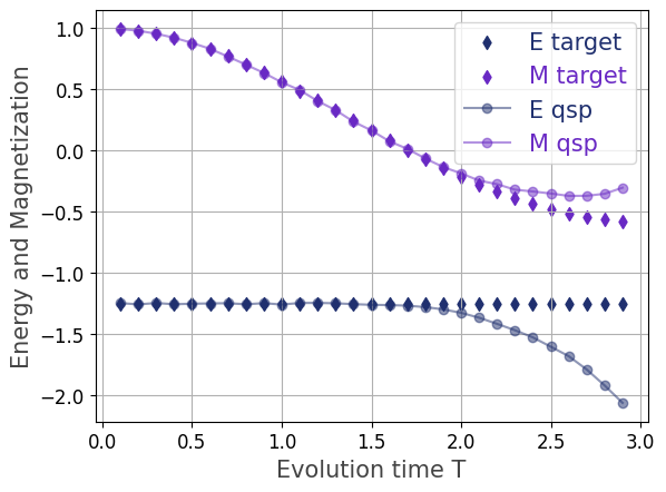
The plots illustrate the time evolution of energy \(E\) and magnetization \(M\) for an Ising model, comparing classical simulation results with those from a quantum simulation employing the Quantum Signal Processing (QSP) based Hamiltonian simulation algorithm.

Analysis of Results

Agreement Phase \(T\le 2.0\): There is excellent agreement between the classical and QSP simulation results for both energy and magnetization during the initial evolution phase, up to an evolution time of \(T=2.0\). The \(M_{\text{qsp}}\) curve closely follows \(M_{\text{classical}}\), while the energy values \(E_{\text{classical}}\) and \(E_{\text{qsp}}\) remain constant as expected for an isolated system.
Divergence Phase \(T>2.0\): Beyond \(T=2.0\), the quantum simulation results diverge noticeably from the classical benchmark. Both \(M_{\text{qsp}}\) and \(E_{\text{qsp}}\) drift away from the classical trajectories, with the energy showing a significant downward trend.
Mitigation: This divergence is attributed to an insufficient truncation order \(N\) used in the QSP polynomial expansion. The simulation error accumulates over time when the truncation order is too low for the required evolution time \(T\). Increasing the truncation order \(N\) can mitigate this effect and maintain accuracy at larger \(T\) values, but this comes at the expense of a higher computational runtime or circuit depth.