qrisp.cks.inner_CKS#

inner_CKS(A, b, eps, kappa=None, max_beta=None)[source]#

Core implementation of the Childs–Kothari–Somma (CKS) quantum algorithm.

This function integrates core components of the CKS approach to construct the circuit: Chebyshev polynomial approximation, linear combination of unitaries (LCU), and qubitization with reflection operators. This function does not include the Repeat-Until-Success (RUS) protocol and thus serves as a subroutine for generating the underlying circuit of the CKS algorithm.

The semantics of the approach can be illustrated with the following circuit schematics:

Implementation overview:

Compute the CKS parameters \(j_0\) and \(\beta\) (CKS_parameters()).
Generate Chebyshev coefficients and unary state angles (cheb_coefficients(), unary_prep()).
Build the core LCU structure and qubitization operator (inner_CKS()).

The goal of this algorithm is to apply the non-unitary operator \(A^{-1}\) to the input state \(\ket{b}\). Following the Chebyshev approach introduced in the CKS paper, we express \(A^{-1}\) as a linear combination of odd Chebyshev polynomials:

\[A^{-1}\propto\sum_{j=0}^{j_0}\alpha_{2j+1}T_{2j+1}(A),\]

where \(T_k(A)\) are Chebyshev polynomials of the first kind and \(\alpha_{2j+1} > 0\) are computed via cheb_coefficients(). These operators can be efficiently implemented with qubitization, which relies on a unitary block encoding \(U\) of the matrix \(A\), and a reflection operator \(R\).

Note

Qubitization requires that the block encoding unitary \(U\) is self-inverse (\(U^2=I\)).

The fundamental iteration step is defined as \((RU)\), where \(R\) reflects around the auxiliary block-encoding state \(\ket{G}\), prepared as the inner_case QuantumFloat.

Repeated applications of these unitaries, \((RU)^k\), yield a block encoding of the \(k\)-th Chebyshev polynomial of the first kind \(T_k(A)\).

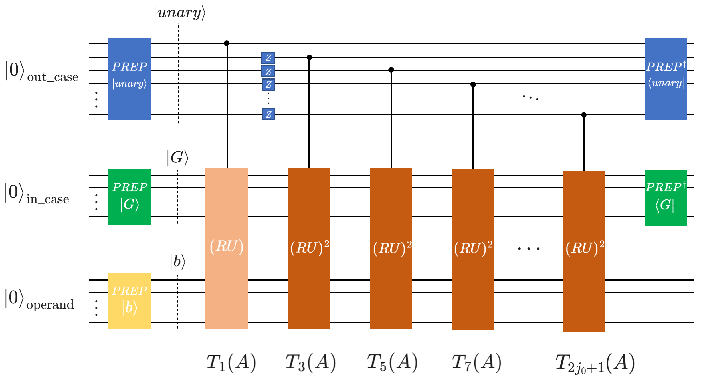
We then construct a linear combination of these block-encoded polynomials using the LCU structure

\[LCU\ket{0}\ket{\psi}=PREP^{\dagger}\cdot SEL\cdot PREP\ket{0}\ket{\psi}=\tilde{A}\ket{0}\ket{\psi}.\]

Here, the \(PREP\) operation prepares an auxiliary out_case Quantumfloat in the unary state \(\ket{\text{unary}}\) that encodes the square root of the Chebyshev coefficients \(\sqrt{\alpha_j}\). The \(SEL\) operation selects and applies the appropriate Chebyshev polynomial operator \(T_k(A)\), implemented by \((RU)^k\), controlled on out_case in the unary state \(\ket{\text{unary}}\). Based on the Hamming-weight \(k\) of \(\ket{\text{unary}}\), the polynomial \(T_{2k-1}\) is block encoded and applied to the circuit.

To construct a linear combination of Chebyshev polynomials up to the \(2j_0+1\)-th order, as in the original paper, our implementation requires \(j_0+1\) qubits in the out_case state \(\ket{\text{unary}}\).

The Chebyshev coefficients alternate in sign \((-1)^j\alpha_j\). Since the LCU lemma requires \(\alpha_j>0\), negative terms are accounted for by applying Z-gates on each index qubit in out_case.

This function supports interchangeable and independent input cases for both the matrix A and vector b from the QLSP \(A\vec{x} = \vec{b}\):

Case distinctions for A

Matrix input:
A is either a NumPy array (Hermitian matrix), or SciPy Compressed Sparse Row matrix (Hermitian matrix). The block encoding unitary \(SEL\) and state preparation unitary \(PREP\) are constructed internally from A via Pauli decomposition.
Block-encoding input:
A is a 3-tuple (U, state_prep, n) representing a block-encoding:
- Ucallable
  Callable U(case, operand) applies the block-encoding unitary \(SEL\).
- state_prepcallable
  Callable state_prep(case) applies the block-encoding state preparatiion unitary \(PREP\) to an auxiliary case QuantumVariable .
- nint
  The size of the auxiliary case QuantumVariable.
In this case, (an upper bound for) the condition number kappa must be specified. Additionally, the block-encoding unitary \(U\) supplied must satisfy the property \(U^2 = I\), i.e., it is self-inverse. This condition is required for the correctness of the Chebyshev polynomial block encoding and qubitization step. Further details can be found here.

Case distinctions for b

Vector input:
If b is a NumPy array, a new operand QuantumFloat is constructed, and state preparation is performed via prepare(operand, b).
Callable input:
If b is a callable, it is assumed to prepare the operand state when called. The operand QuantumFloat is generated directly via operand = b().

Parameters:

Anumpy.ndarray or scipy.sparse.csr_matrix or tuple: Either the Hermitian matrix \(A\) of size \(N \times N\) from the linear system \(A \vec{x} = \vec{b}\), or a 3-tuple (U, state_prep, n) representing a preconstructed block-encoding.
bnumpy.ndarray or callable: Vector \(\vec{b}\) of the linear system, or a callable that prepares the corresponding quantum state.
epsfloat: Target precision \(\epsilon\), such that the prepared state \(\ket{\tilde{x}}\) is within error \(\epsilon\) of \(\ket{x}\).
kappafloat, optional: Condition number \(\kappa\) of \(A\). Required when A is a tuple (block-encoding) rather than a matrix.
max_betafloat, optional: Optional upper bound on the complexity parameter \(\beta\).

Returns:

operandQuantumVariable: Operand variable after applying the LCU protocol.
in_caseQuantumFloat: Auxiliary variable after applying the LCU protocol. Must be measured in state \(\ket{0}\) for the LCU protocol to be successful.
out_caseQuantumFloat: Auxiliary variable after applying the LCU protocol. Must be measured in state \(\ket{0}\) for the LCU protocol to be successful.

Examples

The example shows how to solve a QLSP using the inner_CKS function directly, without employing the Repeat-Until-Success protocol in Qrisp.

First, define a Hermitian matrix \(A\) and a right-hand side vector \(\vec{b}\)

import numpy as np

A = np.array([[0.73255474, 0.14516978, -0.14510851, -0.0391581],
              [0.14516978, 0.68701415, -0.04929867, -0.00999921],
              [-0.14510851, -0.04929867, 0.76587818, -0.03420339],
              [-0.0391581, -0.00999921, -0.03420339, 0.58862043]])

b = np.array([0, 1, 1, 1])

Then, constuct the CKS circuit and perform a multi measurement:

from qrisp.algorithms.cks import inner_CKS
from qrisp import multi_measurement

operand, in_case, out_case = inner_CKS(A, b, 0.001)
res_dict = multi_measurement([operand, in_case, out_case])

This performs the measurement on all three of our QuantumVariables out_case, in_case, and operand. Since the CKS (and all other LCU based approaches) is correctly performed only when auxiliary QuantumVariables are measured in \(\ket{0}\), we need to construct a new dictionary, and collect the measurements when this is true.

new_dict = dict()
success_prob = 0

for key, prob in res_dict.items():
    if key[1]==0 and key[2]==0:
        new_dict[key[0]] = prob
        success_prob += prob

for key in new_dict.keys():
    new_dict[key] = new_dict[key]/success_prob

for k, v in new_dict.items():
    new_dict[k] = v**0.5

Finally, compare the quantum simulation result with the classical solution:

q = np.array([new_dict.get(key, 0) for key in range(len(b))])
c = (np.linalg.inv(A) @ b) / np.linalg.norm(np.linalg.inv(A) @ b)

print("QUANTUM SIMULATION\n", q, "\nCLASSICAL SOLUTION\n", c)
# QUANTUM SIMULATION
# [0.0289281  0.55469649 0.53006773 0.64070521] 
# CLASSICAL SOLUTION
# [0.02944539 0.55423278 0.53013239 0.64102936]

This approach enables execution of the compiled CKS circuit on compatible quantum hardware or simulators.